Factor investing, particularly within the scope of risk premia strategies, has been a popular topic. Vanguard has convinced the investing community that beta can be achieved by buying passive indices and the cost of owning beta should be very low. Investors use risk premia strategies as a source of generating alpha. But, are people looking carefully enough when evaluating these strategies? Much gets hidden in broad risk and return statistics. We thought we would take a deeper dive into how factors behave over market cycles.
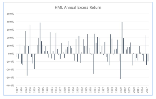
Factor investing is built on the premise that excess returns to stocks can be had by buying stocks that exhibit the factor and shorting those stocks that do not. To test the theory, a factor strategy is back-tested over a sufficiently long historical period and the excess return of the factor over the period is shown along with some statistical information on the robustness of the factor. For example, using the Fama/French 3 Factor monthly data on Professor Kenneth French’s website, since July 1926 the HML factor (High book value to market capitalization stocks versus Low book value to market capitalization stocks, i.e., the value factor) exhibited an annualized 3.8 percent excess return over the entire period. Since 1963, the HML factor exhibited an annualized 3.5 percent excess return over the entire period.
However, excess returns from factors are not stationary, a reality that isn’t clear enough by looking at one number over an entire historical period. Like most investment strategies, excess returns from factor investing go through cycles, periods where the excess returns are quite good and periods where the excess returns are not good at all.
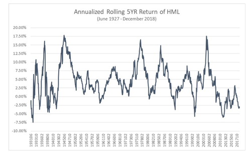
Using the HML factor again, over the historical period available, the annualized rolling 5-year excess return of the factor ranges from up 18 percent to down 8 percent, with most observations occurring in the +12.5 percent to -2.5 percent range. While not shown here, you also see the variability of the HML factor’s excess return in both shorter (e.g., the annualized rolling 3-year excess return) and longer (e.g., annualized rolling 10-year excess return) periods.
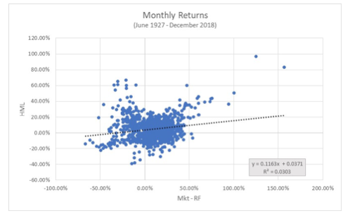
Furthermore, there is hardly any relationship between the rolling 12-month excess return of the HML factor versus the direction of the general equity market (less the risk-free rate or more precisely, the equity risk premium) over the same period. This means that the ex-ante alpha of the value factor should not necessarily be correlated to the equity risk premium return in any 12-month period since there is very little ex-post relationship between the two.
While the benefit of using a single statistic of annualized excess return over the entire historical period is in its simplicity, a more relevant metric would be the distribution of the annualized rolling returns during the historical period as shown here:
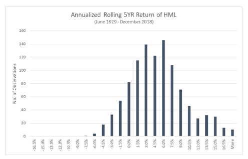
From this distribution chart, you see that over the history of the HML factor, the excess returns of the factor in any 60-month period is usually between 0 percent to 9 percent annualized and the distribution of returns is positively skewed. However, there have been periods where the annualized excess returns of the factor have been negative and a few quite negative.
Quantitative investing strategies are built on testing a strategy over a historical period. The performance of the strategy is typically quantified by the return during the period, the volatility of the return stream, and a risk-adjusted return of the strategy. While this information is relevant, it may be biased by the starting and ending dates used in the analysis. As such, adding a distribution of returns helps an investor frame an appropriate expectation of the performance of the strategy, particularly for out of sample returns.
Kent Huang is chief risk officer at Mount Lucas Management.