


If we reframe the first equation from above in terms of the dividend discount model and relax the assumption of a 100% payout ratio, we are able to see what drives the price-to-book value (BV0 ) multiple:
Since P/E multiples are driven by expected earnings growth, and P/B multiples are driven by expected future Return on Equity (ROE), we will compare current P/E multiples to growth rates and current P/B multiples to ROEs. Exhibit 3 shows these comparisons for the four style factors that we have been examining. We compare the median P/E multiple of extreme quintiles with the respective median rolling FY3/FY1 growth rate**. We also compare the median P/B multiple with the respective median ROE. With these data, we can observe whether the current inter-quintile spread in growth rates explains the spread in P/E multiples, and whether the current spread in ROE explains the spread in P/B multiples. As the formulas above indicate, these relationships are not linear and our analysis does not mean to suggest that they are, however the drivers nevertheless share a direct relationship to the market multiples.
** We acknowledge that the “g” in the equations above is meant to represent growth in perpetuity, however due to data availability and reliability issues with long-term growth (“LTG”) estimates, we rely on FY3/FY1 EPS growth estimates as a proxy.
III. Previous Factor Drawdowns
Finally, in the case of value and momentum specifically, it is helpful to examine the characteristics of past drawdowns for insights into mean reversion trends. Using our proprietary risk model, which strips out the effects of individual styles from country, sector, currency, and idiosyncratic effects, we seek to isolate and link the historical returns attributable to value. These would be the theoretical returns that any portfolio with a pure exposure to value (holding all other factors constant) would have recognized. And as such, we believe they offer a good proxy for the effects impacting value portfolios such as Causeway’s international and global value strategies. Exhibit 4 analyzes the characteristics of previous value drawdowns over the past 25 years (1991 - March 2016) using a broad universe of global equities in the developed markets.
The recent underperformance of value as an investment style has created a strong headwind for value managers, prompting the question, when will value resume its historical outperformance? We seek to answer this question by measuring the magnitude of the current dislocation from three perspectives. We find that value stocks are trading at a much larger discount to their more expensive peers relative to history. They are also much more disconnected from their underlying valuation drivers relative to history. And finally, the drawdown in value has already outpaced the average previous decline. Although recovery could still take longer given the depth of the current drawdown, each of these analyses argue in favor of mean reversion for value. We believe the time to emphasize value has arrived.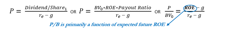
We assume that g = 1 – Payout ratio, so Payout ratio = 1 – g.
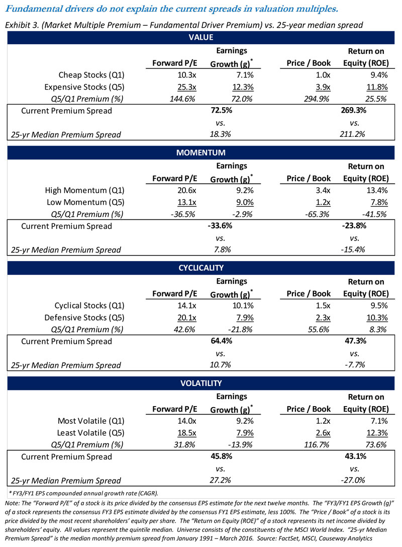
In the cases of value, cyclicality, and volatility, the spread in market multiples far outpaces the spread in the underlying driver. This shows yet again that value stocks, cyclical stocks, and higher-volatility stocks are trading at much bigger discounts to their opposing peers relative to the underlying driver. Admittedly, a valuation premium is probably warranted from more “stable” defensive and low-volatility stocks, but the current valuation spreads are also much greater than their 25-year median spreads (see the boxed comparison). In the case of momentum, high-momentum stocks trade at a much larger premium than the underlying drivers or historical spreads would justify. Again, this is consistent with our conclusions in Exhibit 2.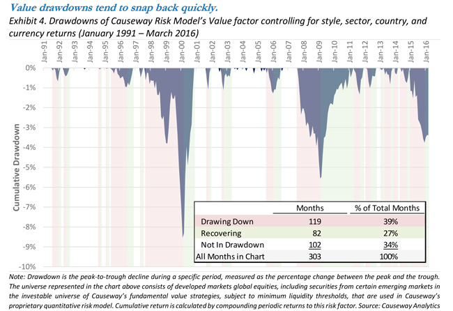
For this analysis, we define a drawdown as any decline lasting two or more months in order to avoid single down months. The average number of months to trough was 6.6 months, and average recovery period was 4.6 months, equating to an average total drawdown period of approximately 11 months. Two observations can be drawn from these statistics. First, we are currently 15 months into a drawdown for value (12 months if the December trough holds), well above the typical trough period of 6.6 months. Second, the average recovery period from a trough is much shorter than the period to the trough. Returns to value tend to recover quickly, which means that attempting to time the bottom may result in a missed recovery. In fact, looking at the table in Exhibit 4, we see that over the past 25+ years, 39% of months were spent drawing down, while only 27% were recovering. This is also consistent with the positive skew in returns to value, indicating that the magnitude of positive returns eclipses the more numerous, smaller declines. Out of the four factors we have discussed, value is the only one with a positive skew (meaning that the other factors experience larger-magnitude negative returns).
Unlike value, momentum has performed very well recently and as contrarian value managers, we have a negative exposure to momentum. However, it is interesting to note that the drawdown pattern is reversed for momentum. Momentum tends to draw down very quickly to its trough, but recovers over a relatively longer period of time. The typical period to trough is 4.9 months compared to the 8.8 month average recovery. Over the past 25+ years, we have witnessed nearly twice as many months in which momentum was recovering than drawing down. Since our value and momentum factors have a -.24 correlation, it is possible that momentum could experience a drawdown at a similar time that value snaps out of a drawdown (and indeed the past several months have witnessed the beginning of a drawdown for momentum). Both would likely be beneficial for Causeway’s developed equity portfolios.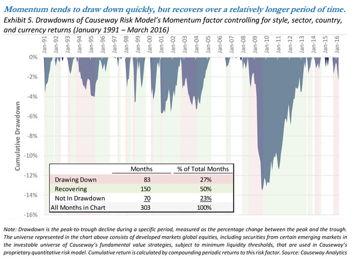
Summary